Divide and Conquer Part 1 (Tiling Puzzle, Binary Search, Merge Sort, Solving Recurrences)
Divide-and-conquer is a powerful algorithmic paradigm. The main ideas behind divide-and-conquer algorithms are as follows.
- We have a problem of size $n$. To solve it, we break it into one or more sub-problems of size smaller than $n$ and solve them recursively.
- Combine the solutions of the sub-problems to solve the original problem.
- When $n$ is small enough (e.g., $\le 1$ or $\le 10$), the problem can be solved directly (base case).
Consider a $2^n$ by $2^n$ ($n \ge 1$) chessboard with one missing square. The task is to tile this board with L-shaped dominoes (2 by 2 with one square removed) such that no two dominoes overlap and no domino goes out of the board’s boundary. See the figure below for an example.
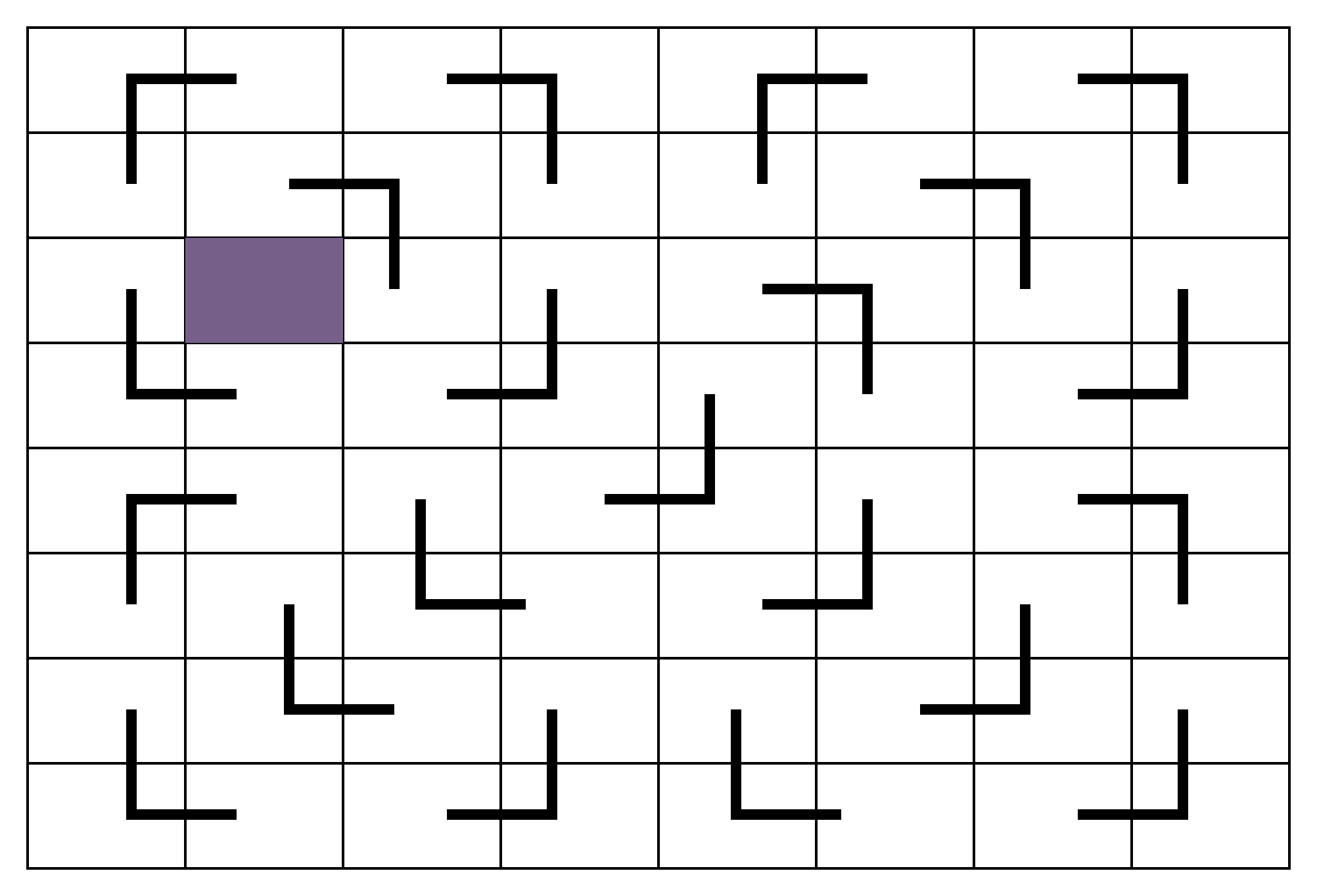
How do we go about solving this problem? One approach is to start with the simplest case that is 2-by-2. This case is trivial since we can orient the domino to avoid the missing square.
Consider the 4-by-4 case. Pause for a while and think about how you would reduce this to the trivial 2-by-2 case.
You can divide the board into four quadrants of size 2-by-2. One of these quadrants has a missing square and you know how to tile it. How about the other three? You can put an L-shaped tile in the center such that it overlaps the other three quadrants. Now, you are left with tiling four 2-by-2 quadrants, each of which has one missing square. Thus, we know how to do this for all 4-by-4 cases.
Can you generalize this to 8-by-8, 16-by-16, and so on?
Let us consider the binary search algorithm. The input is a sorted array of numbers $A[1\ldots n]$ where $A[1] \le A[2] \le \ldots \le A[n]$ and a number $x$. We want to output true if $x$ is in $A$ and false otherwise.
The idea is simple: Look at the middle index $m = \lfloor n/2 \rfloor$. If $x \le A[m]$, then if $x \in A$, it must be in the left half $A[1 \ldots m]$. Otherwise, if it is in $A$, it must be in the right half $A[m+1 \ldots n]$. So we can recursively search either the left half or the right half accordingly. Note that the size of the new sub-problem is now half of the size of the original problem, i.e., $n/2$ vs $n$.
function binary_search(A, x, i, j)
    # Check if x is in A[i:j].
    # Return the index of x if found, otherwise return nothing
    if i == j
        # Base case
        A[i] == x ? return i : return nothing
    else
        m = floor(Int, (i + j) / 2)
        if x ≤ A[m]
            return binary_search(A, x, i, m)
        else
            return binary_search(A, x, m + 1, j)
        end
    end
end

# Initial call
binary_search(A, x, 1, length(A))
What is the running time?
- We start with a search range of size $n$. The search range shrinks by half after each recursion level.
- In each recursion level, there is a constant amount of non-recursive work.
- The search range at recursion level $i$ is $n/2^i$. Solving for $n/2^i = 1$ gives us $i = \log_2 n$.
- The running time is therefore $(\text{# recursion levels}) \times (\text{constant work per level}) = O(\log n) \times O(1) = O(\log n)$.
Often, binary search is implemented iteratively as it is simpler.
# Return the index of x in A if found, otherwise return nothing
function binary_search(A, x)
    i, j = 1, length(A)
    while i < j
        m = floor(Int, (i + j) / 2)
        if x ≤ A[m]
            j = m
        else
            i = m + 1
        end
    end
    return (i ≤ length(A) && A[i] == x) ? i : -1
end
We now look at merge sort which runs in $O(n \log n)$ time. Recall that selection sort runs in $O(n^2)$ time so this is a significant improvement. First, let us look at the merge procedure that merges two sorted arrays $A$ and $B$.
function merge(A, B)
    n, m = length(A), length(B)
    C = Vector{eltype(A)}(undef, n + m)
    ja = jb = j = 1

    while ja ≤ n && jb ≤ m
        if A[ja] ≤ B[jb]
            C[j] = A[ja]; ja += 1
        else
            C[j] = B[jb]; jb += 1
        end
        j += 1
    end

    while ja ≤ n
        C[j] = A[ja];
        ja += 1;
        j += 1
    end

    while jb ≤ m
        C[j] = B[jb];
        jb += 1;
        j += 1
    end

    return C
end
The merge procedure compares the smallest unmerged elements of $A$ and $B$ and appends the smaller one to the end of $C$. This is repeated until all elements from either $A$ or $B$ are merged. Finally, any remaining elements from the other array are appended to the end of $C$. The running time is $O(n+m)$ since each element from $A$ and $B$ is processed exactly once.
Now, we are ready to describe the divide-and-conquer merge sort. Suppose we want to sort $A[1 \ldots n]$. The idea is that we recursively sort $A[1 \ldots \lfloor n/2 \rfloor]$ and $A[\lfloor n/2 \rfloor+1 \ldots n]$ separately and then merge them.
function merge_sort(A)
    n = length(A)
    if n ≤ 1
        return A
    else
        mid = n ÷ 2 # Using integer division for brevity
        L = @view A[1:mid] # @view creates a "view" into A without copying (copy by reference)
        R = @view A[mid+1:end]

        # Recurse and Merge
        sorted_L = merge_sort(L)
        sorted_R = merge_sort(R)

        return merge(sorted_L, sorted_R)
    end
end
The correctness is pretty clear. After recursion, $L$ and $R$ are sorted left and right halves. We merge them to get the sorted array.
Define $T(n)$ as the running time of merge sort on an array of size $n$. Each recursion level does $O(n)$ non-recursive work and calls two sub-problem of half the size. Hence, \(T(n) = 2T(n/2) + O(n).\)
We will show that $T(n)=O(n \log n)$. In fact, $T(n) = \Theta(n \log n)$ is a tighter statement.
Recursion tree
A common way to solve recurrences is to use recursion trees. The idea is to draw a tree where each node corresponds to a call to the function. The running time is the total amount of non-recursive work in the tree.
Example 1: Each level does the same amount of non-recursive work. For example, consider the formula for merge sort: $T(n) = 2T(n/2) + O(n) \le 2T(n/2) + cn$ for some constant $c$. The non-recursive work for a node of size $n$ is $\le cn$.
                          n
                          |
              -----------------------------
              |                           |
             n/2                         n/2
              |                           |
        ---------------             ---------------
        |             |             |             |
       n/4           n/4           n/4           n/4
        |             |             |             |
     --------       --------      --------       --------
     |      |       |      |      |      |       |      |
    n/8    n/8     n/8    n/8     n/8    n/8     n/8    n/8
               ...
- At the 0th level, the amount of non-recursive work is
- At the 1st level, there are two subproblems of size $\frac{n}{2}$, each doing $c\left(\frac{n}{2}\right)$ work. Thus, the total work at this level is
- At the 2nd level, there are four subproblems of size $\frac{n}{4}$; hence, the total work at this level is
This goes on until the base case is reached. At every level of the recursion tree, the total amount of non-recursive work is $c n$. There are at most $O(\log_2 n)$ levels until the recursion reaches the base case. Therefore, the total running time is
\[\boxed{O(n \log n)}.\]Example 2: The non-recursive work done at each level decreases exponentially. For example, $T(n) = T(n/10) + T(n/5) + O(n^2)$.
                              n
                              |
              ---------------------------------
              |                               |
            n/10                            n/5
              |                               |
        ----------------               ----------------
        |              |               |              |
     n/100           n/50           n/50            n/25
        |              |               |              |
    --------        --------        --------        --------
    |      |        |      |        |      |        |      |
 n/1000  n/500   n/500   n/250   n/500   n/250   n/250   n/125
                    ...
- At the 0th level, the amount of non-recursive work is
- At the 1st level, the amount of non-recursive work is
- At the 2nd level, the amount of non-recursive work is
The non-recursive work done at level $i$ is
\[c\left(\frac{1}{20}\right)^i n^2.\]Hence, the total running time is at most
\[\sum_{i=0}^{\log_5 n} c\left(\frac{1}{20}\right)^i n^2 \le \sum_{i=0}^{\infty} c\left(\frac{1}{20}\right)^i n^2 = c n^2 \cdot \frac{1}{1 - \frac{1}{20}} = \boxed{O(n^2)}.\]Here we recall the fact that for $r < 1$,
\[\sum_{i=0}^{\infty} r^i = \frac{1}{1 - r}.\]For example,
\[1 + \frac{1}{2} + \frac{1}{4} + \frac{1}{8} + \cdots = 2.\]Intuitively, the running time is dominated by the work done at the top level, since the work done at each level decreases exponentially.
The missing induction proof. Note that we did not really rigorously prove that the work done at level $i$ is at most $c\left(\frac{1}{20}\right)^i n^2$ (we kind of generalized this fact from the first few levels). This is generally done using induction.
The base case is true since for $i=0$, the work done is at most $c n^2 = c \left(\frac{1}{20}\right)^0 n^2$.
For the inductive step, assume that the work done at level $i$ is at most $c\left(\frac{1}{20}\right)^i n^2$. Each node at level $i$ corresponds to a subproblem of size $s$. The total work done by its two children is at most $c\left(\left(\frac{s}{10}\right)^2 + \left(\frac{s}{5}\right)^2\right) = c\left(\frac{1}{20}\right)s^2$. Let $s_1, s_2, \ldots$ be the sizes of all subproblems at level $i$. Then, the total work done at level $i+1$ is at most
\[\sum_{i} c\left(\frac{1}{20}\right) s_i^2 \le c\left(\frac{1}{20}\right) \left(\sum_{i} s_i^2\right) \le c\left(\frac{1}{20}\right) \cdot \left(\frac{1}{20}\right)^i n^2 = c\left(\frac{1}{20}\right)^{i+1} n^2.\]Example 3: The non-recursive work done at each level increases exponentially. This is a slightly more tricky case, but the rule of thumb is that the work done at the deepest level will dominate the work done by all previous level. For example, consider the following recurrence (which comes up in Strassen’s algorithm for matrix multiplication that we will cover later):
\[T(n) = 7 T(n/2) + n^2.\]Let us again draw the recursion tree.
                                  n
                                  |
        -------------------------------------------------------
        |        |        |        |        |        |        |
      n/2      n/2      n/2      n/2      n/2      n/2      n/2
        |        |        |        |        |        |        |
   --------                     ...                        --------
   |      |                                                |       |
 n/4  ... n/4 (7 times)           ....                    n/4 ... n/4 (7 times)
                         ...
-
Level 0: The amount of non-recursive work is
\(c n^2.\) -
Level 1: There are $7$ subproblems of size $\frac{n}{2}$, each doing
\(c\left(\frac{n}{2}\right)^2\) work. Hence, the total work at this level is \(7c\left(\frac{n}{2}\right)^2 = \frac{7}{4} c n^2.\) -
Level 2: There are $7^2$ subproblems of size $\frac{n}{4}$, each doing
\(c\left(\frac{n}{4}\right)^2\) work. Thus, the total work at this level is \(7^2 c\left(\frac{n}{4}\right)^2 = \left(\frac{7}{4}\right)^2 c n^2.\)Using induction, we can show that the total work done at level $i$ is \(\left(\frac{7}{4}\right)^i c n^2.\)
The recursion has at most $\log_2 n$ levels. The running is therefore at most
\[\begin{align*} c \cdot \sum_{i=0}^{\log_2 n} \left(\frac{7}{4}\right)^i c n^2 & = c \cdot \frac{\left(\frac{7}{4}\right)^{\log_2 n + 1} - 1}{\frac{7}{4} - 1} n^2 \\ & = \Theta \left(n^2 (7/4)^{\log_2 n}\right) \\ & = \Theta \left(n^2 \cdot 2^{\log_2 (7/4) \cdot \log_2 n}\right) \\ & = \Theta (n^2 \cdot n^{\log_2 (7/4)}) = O(n^{2 + \log_2 (7/4)}). \end{align*}\]Numerically, \(2 + \log_2\!\left(\frac{7}{4}\right) \approx 2.807,\) so the final running time is \(\boxed{O\!\left(n^{2.807\ldots}\right)}.\)
Whew!
Master theorem
For most common recurrences, we can directly apply the Master theorem without going through the recursion tree analysis. The proof of the Master theorem is basically a formalization of the recursion tree analysis.
The proof is a formalization of the above examples.
Exercise: Solve the some previous recurrence using Master theorem
- Binary search $T(n) = T(n/2)+O(1)$,
- Merge sort $T(n) = 2T(n/2) +O(n)$,
- Strassen’s algorithm (which we will cover later) $T(n) = 7 T(n/2) + O(n^2)$.
However, Master theorem cannot be used to solve something like this $T(n) = T(n/10) + T(n/5) + O(n^2)$ since it is not in the applicable form. We need to rely on recursion tree in these cases.
Some Other Examples
You should not be over-reliant on Master theorem. Here are some more examples that cannot be solved using Master theorem.
Example: $T(n) = T(\sqrt{n}) + O(1)$ for $n \ge 2$ and $T(n) = O(1)$ for $n < 2$.
Let us draw the recursion tree.
                          n
                          |
                        sqrt(n)
                          |
                       sqrt(sqrt(n))
                          |
                         ...
                          |
                          2
Since each level does $O(1)$ work, we only need to count the number of levels. Let $k$ be the number of levels. Then, we have \(n^{1/2^k} = 2 \implies \frac{1}{2^k} \log_2 n = 1 \implies k = \log_2(\log_2 n).\) Thus, $T(n) = O(\log \log n)$.
Example: $T(n) = T(n-1) + O(n^2)$. We again draw the recursion tree.
                          n
                          |
                         n-1
                          |
                         n-2
                          |
                         ...
                          |
                          1
Each level does $c n^2$ work for some constant $c$. There are $n$ levels. Therefore, the total running time is \(T(n) = c (n^2 + (n-1)^2 + (n-2)^2 + \ldots + 1^2) = \Theta(n^3).\) The last step follows from the formula in the previous chapter.